library(chromConverter)
library(ggplot2)
library(data.table)
#>
#> Attaching package: 'data.table'
#> The following object is masked from 'package:base':
#>
#>     %notin%
MS chromatograms are returned by default in long format
with three columns: retention time, m/z, and intensity.
As an example, we can load the ‘Varian’ SMS chromatogram included in
the chromConverterExtraTests package.
# download example Varian SMS file from the web
path_sms <- tempfile(fileext = ".sms")
download.file("https://raw.github.com/ethanbass/chromConverterExtraTests/master/inst/STRD15.SMS", destfile = path_sms)

dat <- read_chroms(path_sms, format_in = "varian_sms", format_out = "data.frame")
#> Downloading uv...Done!
Plot TIC and mass spectra use base R syntax
x <- dat[[1]]$MS1

# derive TIC using aggregate
tic <- aggregate(intensity ~ rt, data = x, FUN = sum)

# plot TIC
matplot(tic$rt, tic$intensity, type = 'l',
        ylab = "Total intensity", xlab = "Time (min)")
Here is a simple plot function you could use to plot mass spectra using base R graphics:
plot_spec <- function(spec, lab_int=0.2, digits=1){
  plot(spec, type = "h", xlab = "m/z", ylab = "Intensity")
  lab.idx <- which(spec$intensity > lab_int * max(spec$intensity))
  text(spec$mz[lab.idx], spec$intensity[lab.idx], round(spec$mz[lab.idx],
                    digits), offset = 0.25, pos = 3, cex = 0.5)
}
Mass spectra can be extracted by filtering on the time column. For example to get the mass spectrum of the first scan:
times <- unique(x$rt)
spec <- x[x$rt == times[100], -1]
plot_spec(spec)
Plot TIC and mass spectra using dplyr syntax
Plot TIC with dplyr:
tic <- x |> dplyr::group_by(rt) |> dplyr::summarize_at("intensity", sum)

plot(intensity ~ rt, data=tic, type = 'l',
        ylab = "Total intensity", xlab = "Time (min)")
Plot spectrum with dplyr:

Plot TIC and mass spectra using data.table syntax
Convert to data.table:
x <- data.table::as.data.table(x)chromConverter can also return chromatograms in data.table format directly:
dat <- read_chroms(path_sms, format_in = "varian_sms", format_out = "data.table")Extract the total ion chromatogram:
tic <- x[, .(intensity = sum(intensity)), by = rt]
matplot(tic$rt, tic$intensity, type = 'l',
        ylab = "Total intensity", xlab = "Time (min)")
Extract the base ion chromatogram:
bpc <- x[, .(intensity = max(intensity)), by = rt]
matplot(bpc$rt, bpc$intensity, type = 'l',
        ylab = "Base ion chromatogram", xlab = "Time (min)")
To obtain a mass spectrum we just filter by retention time as before:
plot_spec(x[rt == 7.26355, c('mz', 'intensity')])
Plot TIC and mass spectra using ggplot
ggplot(data = tic, aes(x=rt, y=intensity)) +
  geom_line() +
  xlab("Retention time (min)") +
  ylab("Intensity")  +
  theme_minimal()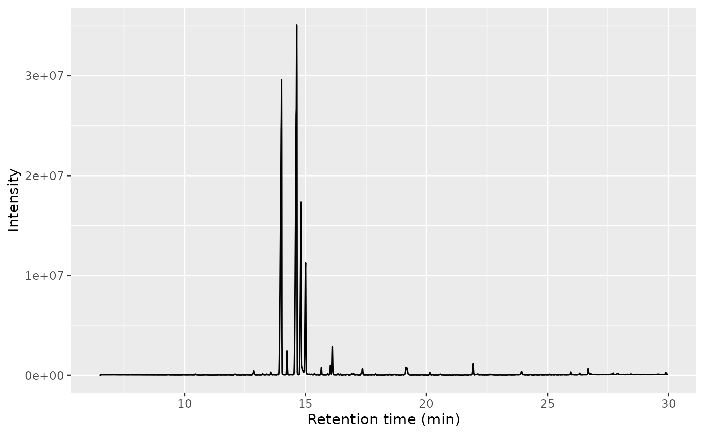
Plot mass spectrum with ggplot:
lab_int <- 0.2
digits <- 1
dplyr::filter(x, rt == 7.26355) |>
  dplyr::select(mz, intensity) |>
  ggplot(aes(x = mz, y = intensity)) +
  geom_segment(aes(xend = mz, yend = 0), linewidth = 0.5) +
  geom_text(data = subset(spec, intensity > lab_int * max(intensity)),
            aes(label = round(mz, digits)),
            vjust = -0.5, size = 2) +
  labs(x = "m/z", y = "Intensity") +
  theme_minimal()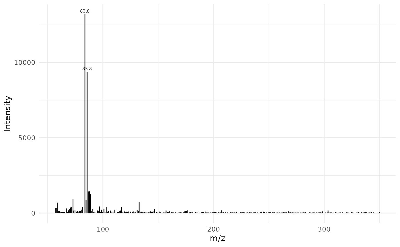
Session Information
sessionInfo()
#> R version 4.6.1 (2026-06-24)
#> Platform: x86_64-pc-linux-gnu
#> Running under: Ubuntu 24.04.4 LTS
#>
#> Matrix products: default
#> BLAS:   /usr/lib/x86_64-linux-gnu/openblas-pthread/libblas.so.3
#> LAPACK: /usr/lib/x86_64-linux-gnu/openblas-pthread/libopenblasp-r0.3.26.so;  LAPACK version 3.12.0
#>
#> locale:
#>  [1] LC_CTYPE=C.UTF-8       LC_NUMERIC=C           LC_TIME=C.UTF-8
#>  [4] LC_COLLATE=C.UTF-8     LC_MONETARY=C.UTF-8    LC_MESSAGES=C.UTF-8
#>  [7] LC_PAPER=C.UTF-8       LC_NAME=C              LC_ADDRESS=C
#> [10] LC_TELEPHONE=C         LC_MEASUREMENT=C.UTF-8 LC_IDENTIFICATION=C
#>
#> time zone: UTC
#> tzcode source: system (glibc)
#>
#> attached base packages:
#> [1] stats     graphics  grDevices utils     datasets  methods   base
#>
#> other attached packages:
#> [1] data.table_1.18.4    ggplot2_4.0.3        chromConverter_0.9.1
#>
#> loaded via a namespace (and not attached):
#>  [1] rappdirs_0.3.4     sass_0.4.10        generics_0.1.4     bitops_1.0-9
#>  [5] xml2_1.6.0         stringi_1.8.7      lattice_0.22-9     digest_0.6.39
#>  [9] magrittr_2.0.5     evaluate_1.0.5     grid_4.6.1         RColorBrewer_1.1-3
#> [13] fastmap_1.2.0      rprojroot_2.1.1    cellranger_1.1.0   jsonlite_2.0.0
#> [17] Matrix_1.7-5       purrr_1.2.2        scales_1.4.0       RaMS_1.4.3
#> [21] pbapply_1.7-4      textshaping_1.0.5  jquerylib_0.1.4    cli_3.6.6
#> [25] rlang_1.3.0        bit64_4.8.2        withr_3.0.3        base64enc_0.1-6
#> [29] cachem_1.1.0       yaml_2.3.12        otel_0.2.0         parallel_4.6.1
#> [33] tools_4.6.1        dplyr_1.2.1        here_1.0.2         reticulate_1.46.0
#> [37] vctrs_0.7.3        R6_2.6.1           png_0.1-9          lifecycle_1.0.5
#> [41] stringr_1.6.0      fs_2.1.0           bit_4.6.0          ragg_1.5.2
#> [45] pkgconfig_2.0.3    desc_1.4.3         pkgdown_2.2.1      bslib_0.11.0
#> [49] pillar_1.11.1      gtable_0.3.6       glue_1.8.1         Rcpp_1.1.2
#> [53] systemfonts_1.3.2  tidyselect_1.2.1   tibble_3.3.1       xfun_0.60
#> [57] knitr_1.51         farver_2.1.2       htmltools_0.5.9    labeling_0.4.3
#> [61] rmarkdown_2.31     compiler_4.6.1     entab_0.3.1        S7_0.2.2
#> [65] readxl_1.5.0